By Nick Bond
It is perhaps belaboring the obvious, but temperatures have increased in WA over the last 50-100 years. From the perspective of extremes, our colder winter months, relative to climatological norms, are not as anomalous as in past decades, and our much warmer than usual months are occurring more frequently. Here we explore how the regional atmospheric circulation relates to monthly mean winter temperatures using neural networks known as self-organizing maps (SOMs).
The SOM framework is being increasingly employed for meteorological and oceanographic applications (Liu and Weisberg 2011). It has been found useful for classifying and visualizing geophysical data, and has some advantages over other analysis methods. It is effective in terms of representing the full continuum of a data set, through its ability to catalog a combination of both common patterns and other states that are rare but distinct. For present purposes, the focus is not on the SOM technique, but rather on some results featuring monthly mean conditions in WA during winter.
Our primary objective is to describe monthly mean circulation patterns in winter as they relate to temperatures and towards that end, a SOM analysis was carried out using two data layers. The first data layer consists of gridded monthly mean 500 hPa geopotential height (Z) anomalies for November through March during the years of 1948 through 2016. The domain encompasses the NE Pacific Ocean, Pacific Northwest and western Canada, specifically, 40-60°N, 145-105°W; the data itself is from the NCEP Reanalysis. The second data layer is monthly mean temperature anomalies for the same months (345 total) from Seattle (KSEA) and Spokane (KGEG). One feature of SOMs is the option to weight the data layers. Here we show results from a SOM trained with weights of 75% for the 500 Z and 25% for the temperatures, since we are most interested in the regional circulation. Other trials revealed that the results were not very sensitive to the weighting. We also constructed SOMs with a variety of configurations, and subjectively settled on a 5×3 matrix (15 patterns). Each pattern is not independent in that the learning procedure leads to an ordered mapping of the input data, considering both data layers, such that neighboring patterns (or nodes) are similar to one another and ones located far apart are more dissimilar.
Composite 500 hPa Z anomaly maps for the months comprising each of the 15 nodes are shown in Figure 1. The central and upper patterns in the far left column (#6 and #11) are accompanied by the coldest temperature anomalies; the three patterns closest to the lower right corner (#4, 5, 10) have the warmest anomalies. The normalized composite temperature anomalies for each pattern at SEA and GEG, and the total number of occurrences of each pattern, are itemized in Table 1. Not surprisingly, low 500 hPa Z heights and anomalous flow from the north imply cold, and high Z and southerly wind anomalies bring warmth. But there are some interesting wrinkles. In a relative sense, the heights are generally more important for temperatures at SEA while the north-south flow anomalies matter more to GEG. An interesting special case is represented by node 15, which has high positive height anomalies, but these months are not warm because they likely include extended periods of settled weather conditions with sinking motion and clear skies resulting in low-level temperature inversions, similar to what we endured for a substantial portion of this past December. Another interesting result regards nodes #11 and 12. The procedure probably separates them mostly because #11 has much colder temperatures than #12, even though their composite height patterns are quite similar. It is difficult to say whether the difference in mean temperatures is due to the modest easterly/ continental component to the anomalous flow in #11 that is absent during the months for #12, or due to some other effect(s), including merely a statistical fluke.
 Figure 1: The 15 composite 500-hPa geopotential height patterns associated with monthly winter (Nov-Mar) temperatures at SEA and GEG identified using the SOM technique. The patterns on the upper left are associated with the coldest temperatures and those on the lower right are associated with the warmest temperatures.
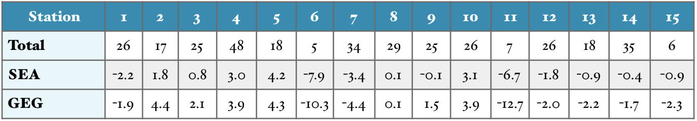 Table 1: Total number of winter months (1948-2016) and mean temperature anomalies (°F) at SEA and GEG for SOM types 1-15.
The frequencies of occurrence of the various nodes vary substantially over the 69-year period of analysis. Time series of the number of months per year of the three warmest patterns (#4, 5, and 10) in Figure 2 indicate that they have occurred throughout the record but have been more frequent in recent decades. Time series of the occurrence of the coldest patterns in Figure 3 reveal a complete absence of the two most extreme nodes (#6 and slightly less rare #11) after 1989. The third coldest and much more common node of #7 has been manifested from time to time in recent years, but somewhat less frequently than earlier in the record.
 Figure 2: The frequency of occurrence for the 3 warmest patterns (#4, 5, 10) identified by the SOM from 1948-2016.
 Figure 3: As in Fig. 2, except for the 3 coldest patterns (#6, 7, 11).
Our interpretation of these findings is that we have not enjoyed an extremely cold month in WA for a long time mostly because of the systematic change in the frequency of occurrence of characteristic regional circulation patterns pertaining to temperatures. It is known that the global climate is changing due to increased greenhouse gas concentrations. What is not clear is whether climate change has been a causal factor in the regional circulation pattern changes seen in this example or whether it’s a coincidence.
Reference:
Liu, Y. and R.H. Weisberg (2011): A Review of Self-Organizing Map Applications in Meteorology and Oceanography, Self Organizing Maps – Applications and Novel Algorithm Design, Dr Josphat Igadwa Mwasiagi (Ed.), ISBN: 978-953-307-546-4, InTech. Available online.