Effect of ENSO on Early Season Snowfall in the Washington Cascades
Most readers of this newsletter are probably aware that El Niño winters tend to result in relatively skimpy snowpacks, and that El Niño development is more likely than not during the upcoming winter. But there is more to it than just that. Keen observers of the climate of the Pacific Northwest (PNW) may know or have noticed that El Niño’s effects often only kick in after the first of the calendar year. We thought it worthwhile to pursue this matter, with two objectives. The first objective is to simply examine the correspondence between El Niño events of modest magnitude (as expected this go around) and early season snowfall in the Washington Cascades. The second is to explore how well an empirical model based on large-scale predictors can account for the variability observed in our snowpack on 1 January. The present piece represents a companion to one published in the January 2016 edition of this newsletter, which also considered ENSO and our weather during the early portion of the cool season.
Our focus will be on the year-to-year variability in a composite measure of snow water equivalent (SWE) on 1 January for the Washington Cascades from 1983-2018. This composite consists of the average SWE at the 5 SNOTEL stations from north to south of Harts Pass, Stevens Pass, Stampede Pass, White Pass, and Lone Pine. We realize that from some perspectives, especially winter sports, snow depth may be of greater interest than SWE. Here we focus on the latter, in part because of the consistency of the data record from the SNOTEL stations used here, and because a reasonable value for the SWE is generally necessary for decent ski conditions in the mountains anyway. Figure 1 shows the time series of composite SWE on 1 January, with the years of weak-moderate El Niño indicated with red dots. The very strong El Niño events of 1982-83, 1997-98 and 2015-16 are not highlighted. There is some ambiguity in the classification of the events for the winters of 1987-88 and 2009-10. We choose to classify the former as moderate-strong (it does not get a red dot) and the latter as moderate (it gets one) on the basis of their expressions in terms of anomalous deep convection in the eastern equatorial Pacific. The main point here is that during past weak-moderate El Niño events there does not seem to be much if any signal in terms of the composite 1 January SWE. While the years of 2003, 2005 and 2015 had SWE values well below average for the period, the years of 1995 and 2007 had values that were well above average. Note also that the greatest SWE back to 1983 occurred in 1997, where the equatorial Pacific was on the cool side but not technically a La Niña, due especially to the large positive anomalies at White Pass and Lone Pine. Figure 1 also includes a set of 3 black diamonds for the year of 2019. These are not observations, of course, but rather forecasts, as detailed below.
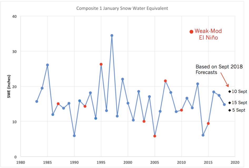
As stated above, we are interested in how well the early season snowfall corresponds with large-scale climate-related variables. Towards that end, a relatively simple empirical model using the generalized additive model (GAM) framework was constructed, with the composite 1 Jan SWE as the predictand. The four predictors included were mean values of the NINO3.4 index during September-November, the regional SST off the coast of the PNW during September, the 500 hPa geopotential height (Z) over WA and OR during November-December, and the 850 hPa zonal wind (U) for western WA and OR during strong (it does not get a red dot) and the latter as moderate (it gets one) on the basis of their expressions in terms of anomalous deep convection in the eastern equatorial Pacific. The main point here is that during past weak-moderate El Niño events there does not seem to be much if any signal in terms of the composite 1 January SWE. While the years of 2003, 2005 and 2015 had SWE values well below average for the period, the years of 1995 and 2007 had values that were well above average. Note also that the greatest SWE back to 1983 occurred in 1997, where the equatorial Pacific was on the cool side but not technically a La Niña, due especially to the large positive anomalies at White Pass and Lone Pine. Figure 1 also includes a set of 3 black diamonds for the year of 2019. These are not observations, of course, but rather forecasts, as detailed below.
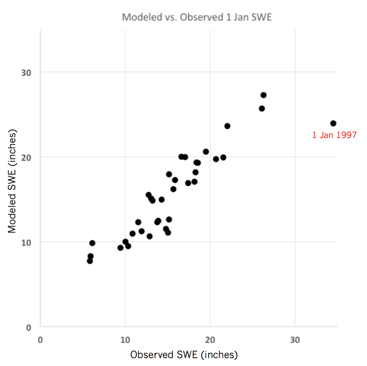
November-December. The main goal here was to explore the strength of the relationships between the predictors and SWE, and secondarily, use those relationships to make some projections for the SWE on 1 January 2019. The GAM framework represents an easy way to assess the relative importance of the predictors. The 500 hPa Z (essentially whether there’s a ridge of high pressure or a trough of low pressure over the PNW) was the big winner, both in terms of the variance in SWE explained and statistical significance. The GAM fit a linear relationship between the 500 hPa Z and the SWE, with lower heights associated with greater SWE. In second place was the 850 U, with greater values tending to be associated with greater SWE, presumably due to stronger onshore flow resulting in heavier precipitation. Of much less importance were the SST anomalies in September off the PNW coast and the NINO3.4 index in September-November. Warmer regional SSTs tend to be followed by a bit less SWE; the weakness in this relationship can probably be attributed to the September SST not being that representative of ocean temperatures later in the winter, and of course, the overriding importance of the regional atmospheric circulation to mountain snowfall. The lack of a relationship between the NINO3.4 index for ENSO and SWE is consistent with the results shown in Figure 1. The GAM based on the four predictors fit the observed SWE quite well (Fig. 2), with the exception of the aforementioned oddball winter of 1996-97.
The GAM discussed above can be run in predictive mode. Using the relationships based on the observational record from 1982-83 through last winter, and observations and forecasts of the 4 predictors, predictions were made for the composite SWE on 1 January 2019. We used a known value for the regional SST in September, relatively short-term forecasts for NINO3.4 in SON from IRI, and forecasts for the 500 hPa Z and 850 hPa U in November-December from NOAA/CPC’s CFSv2 climate model. The latter two predictors are much more important, and uncertain, and therefore we used the data from separate CFS simulations initialized on 5, 10 and 15 September. The resulting 3 individual projections for the 1 January 2019 SWE are shown in Figure 1. All three projections are essentially in the middle of the pack with respect to the observed record back to the early 1980s.
To be sure, these forecasts are mostly for giggles. Additional research would be required to establish the most reliable model(s) for projecting early season snowfall in the Cascades; with GAMs there is the danger of overfitting. On the other hand, we feel that our results justify two takeaway points: ENSO does not seem to be a significant factor, and the mean circulation is a strong determinant, of snow accumulations in the Cascade Mountains during the early winter.